Spark's Execution Model: Drivers, Executors, Stages, and Tasks
Spark’s Execution Model: Drivers, Executors, Stages, and Tasks
You can tune Spark config keys all day and still not fix a slow job if you don’t understand what Spark is actually doing when it runs your code. The single most useful mental model is the one Spark itself uses internally: your DataFrame/RDD code compiles into a directed acyclic graph (DAG) of transformations, and that DAG gets sliced into stages at shuffle boundaries, with each stage running as a wave of parallel tasks across executors.
This post walks through that model. Every claim below traces to the official Spark documentation — config keys to the configuration reference, tuning advice to the tuning guide, the execution model to the cluster overview and SQL programming guide.
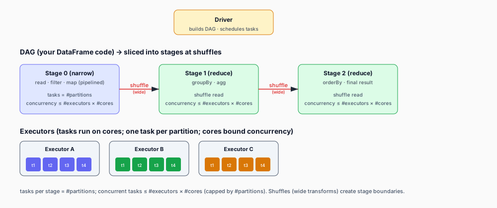
Driver and executors
A Spark application has one driver and one or more executors.
- The driver runs your
mainfunction, builds the SparkSession, compiles your transformations into a DAG, schedules tasks, and tracks their completion. It is the orchestrator. Losing the driver ends the application. - Executors are JVM processes that run on worker nodes. Each executor owns a slice of memory (the executor heap plus memory overhead) and a set of cores (the number of concurrent tasks it can run). Executors fetch tasks from the driver, run them, hold cached/persisted partitions in memory, and write shuffle data to local disk.
A task is the smallest unit of work Spark schedules — it processes one partition of a distributed dataset on one executor core. So the parallelism of a stage is roughly (number of executors) × (cores per executor), bounded above by the number of partitions in that stage.
Partitions: the unit of parallelism
A distributed dataset (RDD, DataFrame, or Dataset) is split into partitions. A partition is a slice of rows that lives on one executor and is processed by one task at a time. The number of partitions in a stage is the ceiling on parallelism for that stage — adding executors beyond the partition count won’t speed that stage up.
Two common partition knobs in the SQL/DataFrame world:
spark.sql.shuffle.partitions— the default number of partitions after a wide transformation (shuffle). Default is 200, which is often too high for small data and too low for large skew-prone data.- Repartitioning operations:
repartition(n)andcoalesce(n)change the partition count.coalescemerges partitions without a full shuffle (good for downsizing before writing);repartitiondoes a full shuffle.
Narrow and wide transformations
Transformations fall into two classes, and the difference is what creates stages.
- Narrow transformations — each input partition contributes to exactly one output partition. Examples:
map,filter,select,withColumnwith a deterministic expression,union. No data moves between executors. These are pipelined within a stage. - Wide transformations — each input partition contributes to multiple output partitions, so data must be redistributed across the network. Examples:
groupBy/agg,join(when not a broadcast or co-partitioned join),distinct,orderBy,repartition. A wide transformation forces a shuffle.
A shuffle is the expensive operation: it writes map-stage output to local disk (shuffle write), the reduce-stage tasks fetch that output across the network (shuffle read), and the whole reduce stage cannot start until the map stage finishes. This is also where most failures concentrate — a FetchFailedException during shuffle read is the classic symptom (covered in the shuffle-fetch-failure post).
How a job breaks into stages
Spark walks the DAG and cuts a stage boundary at every shuffle. The result is a sequence of stages, each containing a run of pipelined narrow transformations ending in (or feeding) a shuffle.
Concretely, for a query like:
result = (
    df.filter(col("amount") > 0)          # narrow
      .groupBy(col("region"))              # wide -> shuffle
      .agg(sum("amount").alias("total"))  # reduce side of the shuffle
      .orderBy(col("total").desc())       # wide -> another shuffle
)
You get something like:
- Stage 0 — read input +
filter(narrow, pipelined). Produces map output written to local disk for the groupBy shuffle. - Stage 1 — shuffle read +
agg(the reduce side of the groupBy). Produces map output for the orderBy shuffle. - Stage 2 — shuffle read + the final ordering.
Within each stage, the number of tasks equals the partition count of that stage’s input. Stages run sequentially when one depends on another (a shuffle dependency); independent stages can run in parallel. You can see all of this in the Spark UI under the Stages tab — task count, shuffle read/write bytes, and the DAG visualization are the diagnostic surface for almost every performance problem.
Why this model matters for tuning
Once you see stages, the common performance fixes fall into place:
- Too few partitions in a stage → underutilized cluster, long tasks, possibly OOM on one executor because a single task holds too much data. Fix: repartition upstream or raise
spark.sql.shuffle.partitions. - Too many partitions → tiny tasks, scheduler overhead dominating. Fix: coalesce.
- Skew — one partition is far larger than the others (e.g. a
groupByon a dominant key). One task runs long while the rest finish; the stage’s wall-clock time equals the slowest task. Symptoms: in the UI, one task’s duration and shuffle read dwarf the rest. Fixes: salt the skewed key, use Adaptive Query Execution (AQE) skew join handling, or pre-aggregate. - Shuffle spill — when shuffle data doesn’t fit in memory it spills to disk; the
disk spillmetric in the UI tells you memory is the bottleneck. - Wide transformations are the cost — reducing the number of shuffles (e.g. avoiding an unnecessary
orderBy, or using a broadcast join for small dimension tables) often beats any memory tuning.
Adaptive Query Execution (AQE)
Since Spark 3, AQE can re-optimize the query plan at runtime, between stages, based on shuffle statistics. Two AQE features directly affect stages:
- Skew join handling — AQE detects skewed partitions from the map-stage shuffle stats and splits the large partition into smaller ones, so the reduce side isn’t dominated by one task.
- Coalescing shuffle partitions — after a shuffle, AQE can merge small partitions post-shuffle so you don’t end up with 200 tiny tasks.
Enabled by default (spark.sql.adaptive.enabled = true). It doesn’t change the stage model — it makes the stage boundaries cheaper.
The takeaway
A Spark job is a DAG sliced into stages at every shuffle, each stage a wave of tasks over partitions running on executors. When a job is slow or failing, the answer is almost always in the Stages tab of the Spark UI: how many tasks, how big is the shuffle, is one task an outlier, did a fetch fail. Config keys tune the edges of this model; understanding the model tells you which key to turn.
Sources & References
- Apache Spark — Cluster Overview (driver, executors, tasks): https://spark.apache.org/docs/latest/cluster-overview.html
- Apache Spark — Configuration (
spark.sql.shuffle.partitions,spark.sql.adaptive.*): https://spark.apache.org/docs/latest/configuration.html - Apache Spark — Tuning (partition sizing, skew, broadcast joins): https://spark.apache.org/docs/latest/tuning.html
- Apache Spark — SQL Programming Guide (DataFrames, AQE): https://spark.apache.org/docs/latest/sql-programming-guide.html
- Apache Spark — Monitoring (Spark UI, stages, task metrics): https://spark.apache.org/docs/latest/monitoring.html